iPlots is a package for the
R
statistical environment (see www.r-project.org)
which provides high interaction statistical graphics, written in Java.
It offers a wide variety of plots, including histograms, barcharts,
scatterplots, boxplots, fluctuation diagrams, parallel coordinates
plots and spineplots. All plots support interactive features, such
as querying, linked highlighting, color brushing, and interactive
changing of parameters. The iPlots package was introduced at
the
DSC-2003
(http://www.ci.tuwien.ac.at/Conferences/DSC-2003/).
The various additions of Version 2.0 were introduced at the
userR!2006 Conference (http://www.r-project.org/useR-2006/).
Besides interactive plots,
iPlots also provides an API for managing plots
and adding user-defined objects, such as lines or polygons to a plot.
Version 2.0 not only adds
new multivariate plots and interactive features throughout all plots,
but also lays the foundations for interactive customizable plots (ICP).
News:
- 2009/07/01 the current development version can be found
here.
The initial release is planned for September this year.
- 2009/04/29 iplots
eXtreme will be presented at the useR!2009
and the DSC2009
meetings and released soon after.
- 2007/08/07 Released iplots_1.1-1 on CRAN.
iSets and iVars are now fully transparent objects and support all usual
opeartions like indexing subsetting etc. as well as sub-assignments.
The latter will use hot-linking, i.e. any changes to the data are
immediately reflected in the plots. See ?iset and ?ivar
in R. Mac users can now use iplots in the console and R GUI (although
somewhat limited) - JGR is still the recommended way.
- 2007/04/18 Released iplots_1.0-8 on CRAN.
Added initial support for (geographic) maps.
- 2006/10/11 Released iplots_1.0-5 on CRAN.
Beside several bugfixes and improved documentation it also features
support for variable-length arguments (e.g. imosaic(AirBags,
Cylinders, Origin) and a more sophisticated registration of iVars
which prevents variable duplication.
- 2006/10/03 Launch of new website, more
documentation will be added gradually.
- 2006/08/20 Release of iplots_1.0-3 (Version
2.0) and binaries for R 2.3.1.
iPlots are now also officially available from CRAN.
- 2006/05/05 Released iplots_0.2-1 (including
Windows and
Mac binaries for R 2.3.0) to go along with JGR. Please note that iPlots
are under continuing development now and features are being added on a
daily
basis, so you may want to update the package evey now and then even if
there is no official release. The next major release is expected for
useR!2006.
- 2005/01/25 Updated webpages; latest versions of
iPlots are available from our R repositories and binaries as a part of
the JGR distribution.
- 2004/06/26 iPlots are now by default delivered with JGR (Java GUI for R). It is
recommended to use iPlots with JGR, because iPlots are seamlessly
integrated into JGR.
Known Bugs and Features:
- View menus need to be cleaned up and consolodated with the context menus.
- More
plot parameters need to be exposed on the R level.
- Some
plots on some platforms do not update properly after creation.
- ...
- Simon
Urbanek
- Tobias
Wichtrey
- Alex
Gouberman
- Martin Theus
(Right now, we mostly use the help-file examples - feel free to contribute!)
Mosaic plots in iPlots are fully interactive, i.e. they not only allow standard selection, highlighting and color brushing but also reordering of variables and the addition and exclusion of variables.
> library(MASS)Here is what you will get:
> data(Cars93)
> attach(Cars93)
> imosaic(data.frame(AirBags,Cylinders,Origin))
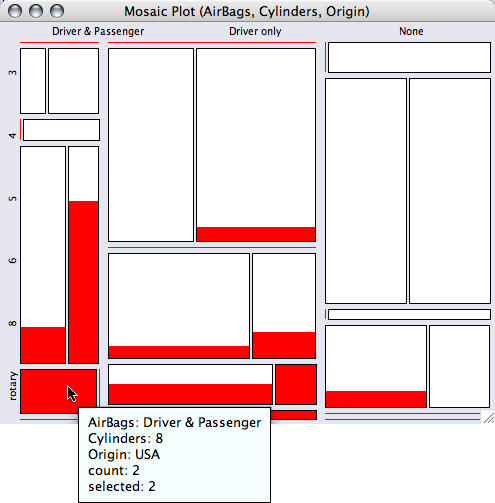
then 200 hp. The query provides exact information for the cell)
- Same Binsize
- Fluctuation Diagram
- Multiple Barchart
- (Model View)
To rearrange the variables use the four arrow keys ... you will soon get the idea of how to manage the variables!
Since most attempts to optimally place labels on mosaic plots fail sooner or later, we use a simple linear spacing for the first variables. Any further information should be queried using <ctrl>-mouse-over.
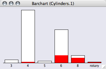
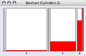
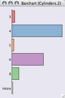
Barcharts in iPlots also feature Spineplots (use ctrl-s or the "View" menu to switch between the two representations)
> library(MASS)yields
> data(Cars93)
> attach(Cars93)
> ibar(Cylinders)
# directly upon creation

> ibar(Cylinders, isSpine=T)

# or switching by changing the plot options of the barchart
# (if no plot is specified, the ibar must be the current plot)

> iplot.opt(isSpine=T)
Bars can be reordered either by using the options in the "View" menu or by <alt>-dragging a bar to its desired position.
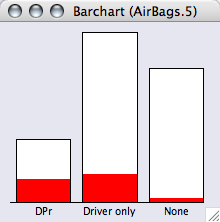
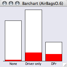
iPlots respect the order of a factor, so orderings from within R can be used to order the categories in a barchart.
> levels(AirBags)
[1] "Driver & Passenger" "Driver only"    "None"

> AirBagsO <- ordered(AirBags,
              c("None", "Driver only", "Driver & Passenger"))

> levels(AirBagsO)
[1] "None"               "Driver only"    "Driver & Passenger"

> ibar(AirBags)
ID:9 Name: "Barchart (AirBags.5)"

> ibar(AirBagsO)
ID:10 Name: "Barchart (AirBagsO.6)"
Interactive maps - which use the data-format of the maptools package - will be availabe soon!
Plots
There is a whole family of parallel plots in iPlots.
I. Parallel Coordinate Plot
A parallel coordinate plot connects all cases by lines.
# Make a PCP for all continuous variables ...The default plot will scale all variables individually between min and max.
> ipcp(Cars93[c(4:8,12:15,17,19:25)])
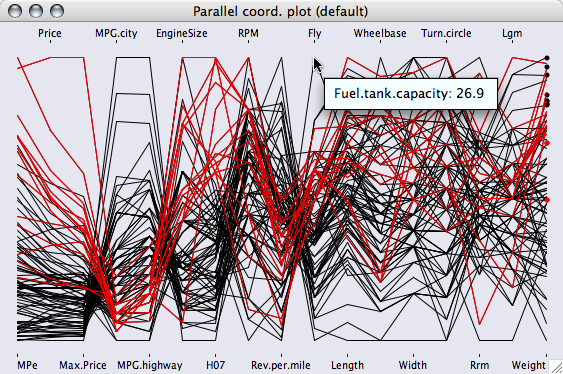
There are various options in the "View" menu including
- Common or individual scale
- Show or hide dots or lines (so a parallel dotplot can be drawn)
- Show only selected cases
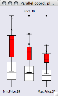
II. Parallel Boxplot
Parallel boxplots are quite similar to PCPs but feature statistics like the median and the hinges, which makes them more useful for comparing distributions of variables.
# Make a parallel boxplot for all price variables ...

> ibox(Cars93[4:6])
 |
 |
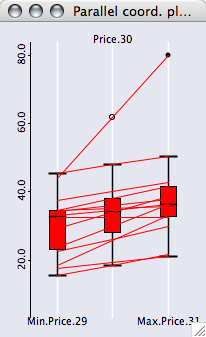 |
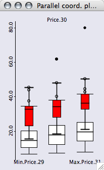
Parallel boxplot for the three prices in the dataset. Each variable uses the full range. |
Using a common scale in the parallel boxplot gives sensible results: max price > price > min price |
Showing only selected cases with the corresponding lines. |
All options can be found in the "View" menu of the plot.
(Note, that the scale is only displayed when all variables share the same scale!)
III. Boxplot y by x
Boxplots y by x are quite different from the two other parallel plots, as they are conditional plots, showing boxplots by group. If ibox() is called with a continuous variable and a factor, a boxplot y by x is created
# split the boxplot for horsepower by number of cylinders

> ibox(Horsepower, Cylinders)
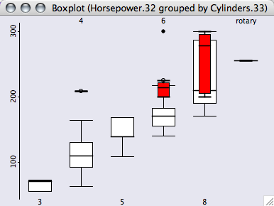
This example shows nicely that all cars having more than 200hp (this is the selected group) have either 6 or more cylinders or a rotary engine. Obviously, a boxplot y by x always uses the same scale for all boxplots for a proper comparison.
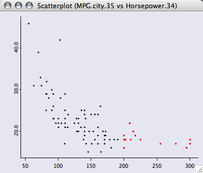
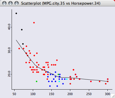
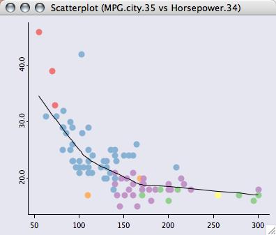
The scatterplot is probably the most frequently used plot of all statistical graphics. Scatterplots in iPlots can be used in the same way as the standard scatterplot in R.
> iplot(Horsepower, MPG.city)
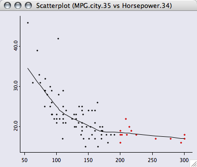
Looking at the above example, a natural step would be to add a scatterplot smoother to the plot.
# create a default lowess smoother

> l <- lowess(Horsepower, MPG.city)

# use ilines() to add the smoother to the iplot()

> ilines(l)
PlotPolygon(coord=1:1,dc=PlotColor(black),fc=none,points=93,...)

# we like to have it a bit rougher, so we remove the first smooth
# and rerun the lowess and plot it again.

> iobj.rm()

> l <- lowess(Horsepower, MPG.city, f=0.5)

> ilines(l)
PlotPolygon(coord=1:1,dc=PlotColor(black),fc=none,points=93,...)
We can also add some additional information to the plot:
# set point size to 5 and color the points by number of cylinders

> iplot.opt(ptDiam=5, col=unclass(Cylinders))
Many other options for the scatterplot within iPlots can be found in the "View" menu.
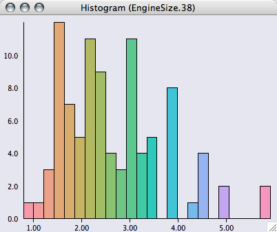
Histograms in iPlots are fully interactive and can also be switched to the spineogram view.
> ihist(Horsepower)
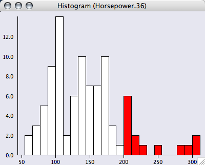
Binwith and anchorpoint can either be changed interactively by <alt>-dragging the leftmost interval border (anchorpoint) or any other bin break (binwidth), or by explicitly specifying the two parameters via iplot.opt() or when creating the plot.
> iplot.opt(anchor=25, binw=25)
Histograms rescale by default when their parameters are changed, which can be controlled by two flags (see the help pages for details).
Selection in all iPlots can be done via selecting single objects like a point, a bar/rectangle or a line, or by creating a drag-box, which selects all points within the rectangle.
Via the iset-functions, the selection state of an iplot session can be queried and modified.
# get selected indices
> iset.selected()
[1] 76 63 59 52 30 10 5 2 50 57 48 11 28 19
# what proportion of the dataset is selcted?
> sum(sign(iset.selected()))/length(Horsepower)
[1] 0.1505376
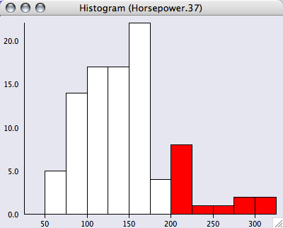
# select all cases for cars with more than 150hp
> iset.select(Horsepower >= 150)
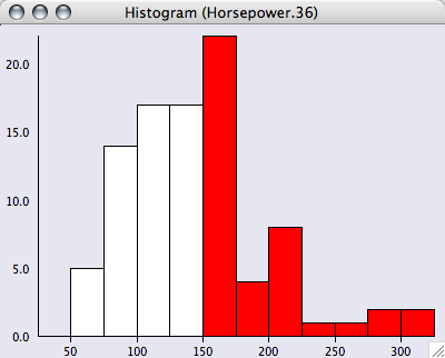
All plots, which share the same iset are updated immediately.
To perform more complex selections, pressing the <shift>-modifier will select data in XOR mode.
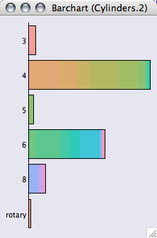
Selections are a transient attribute of the data. Whenever a new selection is defined, the old selection state is overwritten. A persistent color attribute can be defined using color brushing within iPlots.
Color brushing can either be applied via the col=... option in iplot.opt() or any other iPlot graphics, or via the "View > Set Colors (CB)" menu command.
The same could be done from within R (though using the standard R colors) with:
# set colors according to Cylinders (using standard R colors)A second option for using color brushing is to apply rainbow colors over the range of a continuous variable. The menu command "View > Set Colors (rainbow)" will set the color scheme.
> iplot.opt(col=unclass(Cylinders))
WIth iObjects you can annotate plots with further graphical elements. iObjects are
- ilines()
- itext()
- iabline()
# create the scatterplot

iplot(EngineSize, Horsepower)

# select all but the outliers, save the selection subset for
# the regression

> subs <- iset.selected()

# add the linear regression to the scatterplot

> iabline(lm(Horsepower ~ EngineSize, subset=subs))
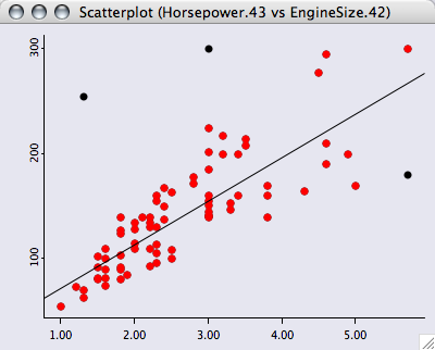
Not really a good model, but at least we got rid of the outliers very easily.
There are some housekeeping functions for iObjects (please refer to the help files for details).
- iobj.cur()
- iobj.get()
- iobj.list()
- iobj.next()
- iobj.opt()
- iobj.prev()
- iobj.rm()
- iobj.set()
Interactive graphics benefits strongly from an interface which is highly consistent and has a flat learning curve. The most important functionality within iPlots are the keyboard shortcuts and modifier keys.
- <shift>-selection is always in XOR-mode
- to query an object or plot canvas, mouse-over while <ctrl> is pressed
- <command>-drag-box
(MAC), middle mouse button zooms in and out
(to zoom out, just click, i.e. a zero size drag-box) - <command>-r / <ctrl>-r rotates plots
Many other common functions can be found in the "View" menu.
The handling of iPlots is done via a set of maintenance functions (see help files for details). The basic concept follows the handling of devices within R. It is, however, advisable to use plot objects directly, especially in scripts.
- iplot.cur()
- iplot.data()
- iplot.list()
- iplot.new()
- iplot.next()
- iplot.off()
- iplot.opt()
- iplot.prev()
- iplot.set()
- iset.brush()
- iset.col()
- iset.cur()
- iset.df()
- iset.list()
- iset.new()
- iset.next()
- iset.prev()
- iset.sel.changed()
- iset.select()
- iset.selectAll()
- iset.selected()
- iset.selectNone()
- iset.set()
The α-channel can be used to specify the transparency of a painted object. This is useful, when plotting very many objects , which would otherwise result in heavy overplotting. Thus the density of objects can be easily displayed.
All glyph-based plots in iPlots offer α-channel transparency to handle large data and avoid
overplotting.
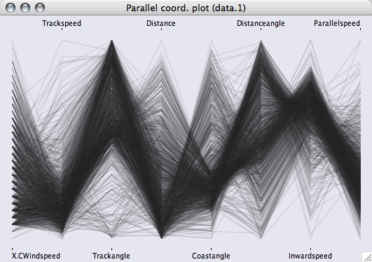
(α-transparency
in parallel coordinate plots)
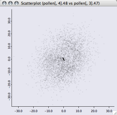
(α-transparency in a scatterplot - you recognise the dataset?!)
Use the arrow keys
(left and right) to interactively increase or decrease the transparency.
Where can I download iPlots?
- The current version of iPlots for R
can be downloaded from CRAN. Use either the package manager from
your favorite GUI or type: install.packages("iplots",dep=TRUE)
- The latest source packages can be found in our R repositories:
- Release repository (CRAN): iPlots
at CRAN
This repository also feature binary packages for Windows and Mac OS X - RForge repository: http://www.rforge.net/iplots/files
Is there anything else I need to install in order to use iPlots?
For other UNIX operating systems (in particular Linux) Sun Java 1.5 or higher is highly recommended (64-bit Linux requires at least Java 1.6 beta). For the best user-experience, iPlots can be run from within JGR.
rJava fails to load on Unix, what can I do?
Error in dyn.load(x, as.logical(local), as.logical(now)) :then your R was configured without Java support. To enable Java support in R, make sure you have installed R 2.4.0 or higher, Java works (e.g. java -version) and run as root:
unable to load shared library '/usr/lib/R/library/rJava/libs/rJava.so':
libjvm.so: cannot open shared object file: No such file or directory
R CMD javareconf
Please post questions and bug reports to the mailing list stats-rosuda-devel.
Issues of general interest will be posted on this page.